3  Pre-workshop tasks

Warning

🚧 We are doing major changes to this workshop, so much of the content will be changed. 🚧

In order to participate in this workshop, you must complete this section for the pre-workshop tasks and finish with completing the survey at the end. These tasks are designed to make it easier for everyone to start the workshop with everything set up. For some of the tasks, you may not understand why you need to do them, but we hope by the start of the workshop (and by the end) that you understand them better.

These tasks could take between 2-6 hrs to finish depending on:

• Your current skill and knowledge level when it comes to computers, installing programs, and experience from taking our other workshops or ones that are similar to them.
• If you will be using a work laptop and if your institution has more restrictive policies on what you can install on your computer. You may need to contact your work IT sooner than later for help or to get permissions. From our experience, this can be the hardest part of these pre-workshop tasks since it can be out of your control.

So, we suggest you plan at least a full day to complete these pre-workshop tasks and that you start them sooner than later.

3.1 List of tasks

Here’s the list of tasks you need to do. Specific details about them are found as you work through the tasks.

1. Read Section 3.2 for the learning objectives for the pre-workshop tasks.
2. Read on how to read this website in Section 3.3.
3. Follow the installation instructions in Section 3.4. Install a version of R, RStudio, and Git that is as updated as possible.
4. Install the necessary R packages in Section 3.5.
5. Read about Git from the introduction workshop and configure Git on your computer in Section 3.6. If you haven’t used Git before, this task could take a while because of the reading.
6. Confirm your Git setup in Section 3.7. This is a check to see if everything is working correctly. You’ll later need to paste this output into the survey.
7. Create an R Project in Section 3.8, including the folder and files.
8. Create a Quarto file in Section 3.9.
9. Download the data in Section 3.10 and save it to your computer. Run a check in this subsection to see that everything is as expected. You’ll later need to paste this output into the survey.
10. Read about the basic workshop details in Section 3.11.
11. Read the syllabus in Chapter 1.
12. Read the Code of Conduct.
13. Complete the pre-workshop survey. This survey is pretty quick, maybe ~10 minutes.

Check each section for exact details on completing these tasks.

3.2 Learning objectives

In general, these pre-workshop tasks are meant to help prepare you for the workshop and make sure everything is setup properly so the first session runs smoothly. As part of the preparation, some of the tasks that you need to do are some learning and reading about concepts we use throughout the workshop but that don’t directly cover. These readings will best prepare you and your fellow learners for the workshop. So the learning objectives for this section will enable you to:

1. Recall (or describe) what reproducible documents are and what Quarto is.
2. Describe more details about what a filesystem is, what relative and absolute paths are, and how to make use of them with the fs and here R packages to navigate files in your project.
3. Use functions to download and begin to organise raw data for your project.
4. Recall (or describe) the basics of Git and how to configure it on your computer.

3.3 Reading the workshop website

We will explain this a bit more during the workshop, but read this section to know how to read certain things on the website. Specifically, there are a few “syntax” type formatting of text on the website to know about:

• Folder names always end with a /, for example data/ means the data folder.
• File names always end with their file extension, for example content.md means the file is a Markdown file.
• R variables are always shown as is. For instance, for the code x <- 10, x is a variable because it was assigned with 10.
• Functions always end with (), for instance mean() or read_csv().
• Sometimes functions have their package name appended with :: so that you run the code from the specific package, since we likely haven’t loaded the package with library(). For instance, to install packages from GitHub using the pak package we use pak::pak("user/packagename"). You’ll learn about this more later.

3.4 Installing the latest programs

In order to participate in the workshop, you’ll need to install these programs. You may already have some of them installed and if you did, please make sure that they are at least the minimum versions listed below. If not, you will need to update them.

Windows

1. R: Any version above 4.4.0. If you have used R before, you can confirm the version by running R.version.string in the Console.
2. RStudio: Any version above v2024.04.2+764. If you have installed it before, check the current version by going to the menu Help -> About RStudio.
3. Git: Select the “Click here to download” link. Git is used throughout many sessions in the workshop. When installing, it will ask for a selecting a “Text Editor” and while we won’t be using this in the workshop, Git needs to know this information so choose Notepad.
4. Rtools: Version that says “R-release”. Rtools is needed in order to build some R packages. For some computers, installing Rtools can take some time.

MacOS

1. R: Any version above 4.4.0. If you have used R before, you can confirm the version by running R.version.string in the Console. If you use Homebrew, installing R is as easy as opening a Terminal and running:

   brew install --cask r

2. RStudio: Any version above v2024.04.2+764. If you have installed it before, check the current version by going to the menu Help -> About RStudio. With Homebrew:

   brew install --cask rstudio

3. Git: Git is used throughout many sessions in the workshop. With Homebrew:

   brew install git

Linux (Ubuntu)

1. R: Any version above 4.4.0. If you have used R before, you can confirm the version by running R.version.string in the Console.

   sudo apt -y install r-base

2. RStudio: Any version above v2024.04.2+764. If you have installed it before, check the current version by going to the menu Help -> About RStudio.

3. Git: Git is used throughout many sessions in the workshop.

   sudo apt install git

All these programs are required for the workshop, even Git. Git, which is a software program to formally manage versions of files, is used because of it’s popularity and the amount of documentation available for it. Check out the online book Happy Git with R, especially the “Why Git” section, for an understanding on why we are teaching Git. Windows users tend to have more trouble with installing Git than macOS or Linux users. See the section on Installing Git for Windows for help.

Note

Some pictures may show a Git pane in RStudio, but you may not see it. If you haven’t created or opened an RStudio R Project (which is taught in the introductory workshop), the Git pane does not show up. It only shows up in R Projects that use Git to track file changes.

Note

A note to those who have or use work laptops with restrictive administrative privileges: You may encounter problems installing software due to administrative reasons (e.g. you don’t have permission to install things). Even if you have issues installing or updating the latest version of R or RStudio, you will likely be able to continue with the workshop as long as you have the minimum version listed above for R and for RStudio. If you have versions of R and RStudio that are older than that, you may need to ask your IT department to update your software if you can’t do this yourself. Unfortunately, Git is not a commonly used software for some organizations, so you may not have it installed and you will need to ask IT to install it. We require it for the workshop, so please make sure to give IT enough time to be able to install it for you prior to the workshop.

Once R, RStudio, and Git have been installed, open RStudio. If you encounter any troubles during these pre-workshop tasks, try as best as you can to complete the task and then let us know about the issues in the pre-workshop survey. If you continue having problems, indicate on the survey that you need help and we can try to book a quick video call to fix the problem. Otherwise, you can come to the workshop 15-20 minutes earlier to get help.

If you’re unable to complete the setup procedure due to unfixable technical issues, you can use Posit Cloud (to use RStudio on the cloud) as a final solution in order to participate in the workshop. For help setting up Posit Cloud for this workshop, refer to the Posit Cloud setup guide.

3.5 Installing the R packages

We will be using specific R packages for the workshop, so you will need to install them. A detailed walkthrough for installing the necessary packages is available on the pre-workshop tasks for installing packages section of the introduction workshop, however, you only need to install the r3 helper package in order to install all the necessary packages by running these commands in the R Console:

1. Install the pak package:

   install.packages("pak")

2. Install our custom r3 helper package for this workshop:

   pak::pak("rostools/r3")

3. Install the necessary packages for the workshop:

   r3::install_packages_intermediate()

Warning

You might encounter an error when running this code. That’s ok, you can fix it if you restart R by going to Sessions -> Restart R and re-run the code in items 2 and 3, it should work. If that also doesn’t work, try to complete the other tasks, complete the survey, and let us know you have a problem in the survey.

Note: When you see a command like something::something(), for example with r3::install_packages_intermediate(), you would “read” this as:

R, can you please use the install_packages_intermediate() function from the r3 package.

The normal way of doing this would be to load the package with library(r3) and then running the command (install_packages_intermediate()). But by using the ::, we tell R to directly use a function from a package, without needing to load the package and all of its other functions too. We use this trick because we only want to use the install_packages_intermediate() command from the r3 package and not have to load all the other functions as well. In this workshop we will be using :: often.

3.6 The basics of Git

Since Git has already been covered in the introduction workshop, we won’t cover learning it during this workshop. However, since version control is a fundamental component of any modern and reproducible data analysis workflow and should be used, we will be using it throughout the workshop.

Important

If you have used or currently use Git, you can skip this section and move on to Section 3.7.

Git itself isn’t too difficult to use. But the concepts that Git uses are very difficult to learn and use. That’s because Git requires you to view your files and folders and computer very differently to how you may normally be used to working with them. And because we will be using Git throughout the workshop, to ensure you have the smoothest experience, we want you to at least be aware of and have read a bit about Git. So, from the introduction workshop, please read these sections:

1. What is version control?
2. What is Git?
3. Basics of Git

After reading them, in your RStudio in the R Console, run this function that should open up a pop-up window to type in your name and email:

Console

r3::setup_git_config()

For most of the workshop, we will be using Git as shown in the Using Git in RStudio section. Later on during the workshop, we might connect our projects to GitHub, which is described in the Synchronizing with GitHub section.

3.7 Confirming your Git setup

Since you will be using Git regularly throughout the workshop, please run this check to ensure everything is setup correctly. Type and run this function in the R Console of RStudio:

Console

r3::check_setup()

The output you’ll get for success should look something like this:

Checking R version:
✔ Your R is at the latest version of 4.4.0!
Checking RStudio version:
✔ Your RStudio is at the latest version of 2024.12.1.563!
Checking Git config settings:
✔ Your Git configuration is all setup!
  Git now knows that:
  - Your name is 'Luke W. Johnston'
  - Your email is 'lwjohnst@gmail.com'

Eventually you will need to copy and paste the output into one of the survey questions.

Note

While GitHub is a natural extension to using Git, given the limited time available in the workshop, we will not be going over how to use GitHub. If you want to learn about using GitHub, check out this session about it in the introduction workshop.

3.8 Create an R Project

One of the first, basic steps to ensuring a reproducible and modern data analysis workflow is to keep everything self-contained in a single location. In RStudio, this is done by using R Projects. Read all of this reading task from the introduction workshop to learn about R Projects and how they help keeping things self-contained. You don’t need to do any of the exercises or activities.

Caution

Depending on your institution’s policies or procedures, you may have some type of file synching software like OneDrive or Dropbox installed on your computer and your IT may have set it up so that (nearly) all your files and folders are synched through this software. Sometimes IT has set it up so it is fairly straightforward to not use it, but often, it can be extremely difficult to find a folder that isn’t being synched. This is usually the case for Windows users and less for MacOS users, but they can sometimes have these programs installed and setup for them too.

Unfortunately, these types of software can cause very subtle, small issues when working with Git, R, and RStudio that are very difficult to troubleshoot, for both you and for us as the instructors. They cause these subtle issues because they are constantly working to synchronize files and folders. This can sometimes cause conflicts with files when using Git and especially when doing more data intensive work that creates and deletes many files often. You may also notice that your computer is slower when working with R and RStudio while using these synched folders. That’s because of the constant synching of files. It isn’t the fault of R and RStudio, but is instead because of the synching software.

A related issue is when you store your files on a shared drive, like H: or E: or U: drives on Windows. This is again because your institution may have a procedure for using these folders to “more easily share with colleagues” or to keep everything on their servers. But these shared drives have a very similar issue as using Dropbox or OneDrive, because they also have to continually upload and download over the internet from your computer to your work’s remote server. Any time your computer needs to regularly communicate over the internet, like when using files stored on a server in the shared drives, things will be slower. So, you may feel like RStudio is slow, but it is actually because of the way your computer has been setup by your IT.

So in general, we tend to strongly recommend not creating your R projects in these synched folders or in these shared drives. We’ve learned that many, common problems we encounter during the workshops are because of these synched folders or shared drives. That’s why we will be getting you to create your R Project on your Desktop on your computer (not shared drive). Usually, but not always, this folder is not tracked by these synching programs.

So find the path to your Desktop folder at C:\Users\yourusername\Desktop\ for Windows users and /Users/yourusername/Desktop/ for MacOS and use that as the location for your R Project.

There are several ways to organise a project folder. You’ll be using the structure from the package prodigenr. The project setup can be done by either:

1. Using RStudio’s New Project menu item: “File -> New Project -> New Directory”, scroll down to “Scientific Analysis Project using prodigenr” and name the project “LearnR3” in the Directory Name, saving it to the “Desktop” as described above with Browse. When you use this method, the new RStudio Project will automatically open up for you.
2. Or, running the function prodigenr::setup_project("~/Desktop/LearnR3") in the R Console. The ~ is a shortcut for your home directory, so this function will create a new folder called LearnR3 on your Desktop. When you use this method, you will need to use your file manager to navigate to the Desktop folder and open the LearnR3.Rproj file inside of the newly created LearnR3/ folder.

After opening the new RStudio Project, run this next function in the R Console to create a new R script file called functions.R in the R/ folder. This is where you will be moving all the functions that you will create during the course.

Console

usethis::use_r("functions", open = FALSE)

Here you use the usethis package to help set things up. usethis is an extremely useful package for managing R Projects and we highly recommend checking it out more to see how you can use it more in your own work.

3.9 Quarto

We teach and use Quarto (which is a more powerful, next generation version of R Markdown) because it is one of the very first steps to being reproducible and because it is a very powerful tool for doing data analysis. Please do these two tasks:

1. Read over the Quarto section of the introduction workshop. If you use Quarto already and are familiar with it, you can skip this step.

2. If you are not already in the LearnR3 project, open it up by either clicking the LearnR3.Rproj file in the LearnR3/ folder or by using the “File -> Open Project” menu. Run the function below in the Console when RStudio is in the LearnR3 project, which will create a new file called learning.qmd in the docs/ folder.

   Console

   r3::create_qmd_doc()

Throughout the workshop, you will use this document to build up and run your code, as well as to prototype the functions you’ll create before you move them into the functions.R file.

3.10 Download the workshop data

To best demonstrate the concepts in the workshop, it’s best to use a real dataset to apply what you’re going to learn. So for this workshop, you’re going to use an openly licensed dataset from a study looking at how bioactive components in food impact our gut microbiota, which is called the DIME study (1).

1.

Traka M, Omieljaniuk M, Ahn-Jarvis J, Bernuzzi F, Ng DYK. The effect of dietary bioactive on gut microbiome diversity (DIME) – a pilot study. Zenodo; 2023.

Unfortunately, like most research data, it isn’t the most tidy. So it’s been cleaned up a bit for you to use in this workshop.

Tip

Much of the concepts and skills we will cover in this workshop were used to process and prepare this dataset for you to use in this workshop. If you want to see the code “in action”, check out the data-raw/dime.R script in this workshop’s GitHub repository.

Since this workshop is about being reproducible and applying modern approaches to data analysis, you’re going to start by writing and saving R code to download the dataset your R project and save it to a folder called data-raw/. During the workshop we’ll be continuing to process and prepare this dataset for analysis, though we won’t do any statistical analysis during this workshop.

The end goal for this workshop is that you will have a sequence of R code written within the Quarto document that will take this raw data and process it into a cleaned and prepared dataset. Processing data for cleaning is something that you will do a lot of in your own work, since most research data is not directly ready to be analysed. In the process of processing the data, you’ll also learn concepts and skills that can be applied to many different tasks and situations.

For now, read the description of the DIME dataset that was taken from the DIME dataset page:

“The DIME study consists of a randomised 2x2 cross-over human intervention where healthy participants (n = 20) are subjected to a diet high in bioactive-rich food for two weeks and a diet low in bioactive-rich food. There is a four-week washout between the two interventions.

The continuous glucose monitoring was achieved using the Abbott [freestyle] libre flash glucose device. The baseline of the participants were determined 7 days before the start of the intervention, followed by the first arm and second arm. The period between the two arms (washout) was not recorded.

We also included sleep data which consists of the amount of time spent in bed and during that time the amount of time spent in light, deep and rem in all 20 participants during the course of the dietary intervention, both the high and low bioactive diet. that was captured using [FitBit] wearables during both stages of the dietary intervention”

Note

You may be wondering, how can we be using this dataset that has human health data? Isn’t that against GDPR? The short answer is no, it isn’t.

If you went to the dataset page, you may have noticed that the dataset is openly licensed and public, which means you can use it for your own purposes. Yes, it is possible to openly license and make health data publicly available! And no it doesn’t conflict with privacy laws like GDPR. Unfortunately, the way that universities have communicated about GDPR’s impact on and role in research data hasn’t been done very well. They’ve communicated things in a very alarmist, risk-averse way and made their recommendations or policies so generalised to the point of not being useful to specific situations.

So, while GDPR does make it more strict on what can and cannot be shared and requires more detailed information on how the participant’s data will be used when getting prior informed consent, it does not prohibit sharing it or making it public! GDPR and open data are not strictly in conflict with one another.

The standard and conventional way of saving raw data in R is to save it to the data-raw/ folder. There is a helper function for that from usethis. While in your LearnR3 R Project, go to the R Console pane in RStudio and type out:

Console

usethis::use_data_raw("dime")

What this function does is create a new folder called data-raw/ and creates an R script called dime.R in that folder. This is where we will store the mostly raw (though partly cleaned up) DIME data that you’ll get from the workshop’s GitHub repository. After running this function, the R script should open up for you, otherwise, go into the data-raw/ folder and open up the new dime.R script.

The first thing you want do is delete all the code in the script that is added there by default. Then write this library() function at the top of the file:

data-raw/dime.R

library(here)

Tip

The here package was described in the Import data session of the introductory workshop and makes it easier to refer to other files in an R project. Read through the section about the here package in the introductory R workshop to learn more.

R runs code while working in the current working directory, which you can see on the top of the RStudio Console pane and is shown in the red box inside the image below.

The folder location that R does it’s “work”, called the “working directory”, highlighted by the red box.

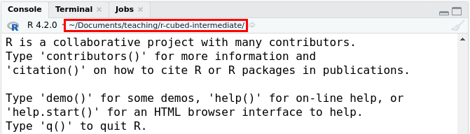
When in an RStudio R Project, the working directory is the folder where the .Rproj file is located. When you run scripts in R with source() or when you render a Quarto document, sometimes the working directory will be set to the folder that the R script or Quarto document is located in. So you can sometimes encounter problems with finding files if your code needs to load or use a file and you don’t use a function like here() to link to it. When you use here() it tells R to start searching for files from the .Rproj location.

Let’s use an example. Below is the list of the folders and files you have so far in your R Project.

.
├── DESCRIPTION
├── LearnR3.Rproj
├── R
│   ├── README.md
│   └── functions.R
├── README.md
├── TODO.md
├── data
│   └── README.md
├── data-raw
│   ├── README.md
│   └── dime.R
└── docs
    ├── README.md
    └── learning.qmd

Note

You don’t need to run the below code. But if you want to see the structure and content of a directory, you can use the dir_tree() function from the fs package, which means “filesystem”, by running the following code in the R Console:

Console

# To print the file list.
fs::dir_tree("~/Desktop/LearnR3", recurse = 1)

If we open up RStudio with the LearnR3.Rproj file and run code in the data-raw/dime.R, R runs the commands assuming everything starts in the LearnR3/ folder. But! If we run the code that is in the dime.R script by, e.g. not while in RStudio, not in the R Project, or using source(), R runs the code in that file by assuming the working directory is the folder that the file is in, which is in the data-raw/ folder. So if you try to load in data in another folder like data/, R will think you mean the data/ folder in the data-raw/ folder, which doesn’t exist! So this can make things tricky. What here() does is to tell R to first look for the .Rproj file and then start looking for the file we actually want. This might not make sense yet, but as we go through the workshop, you will see why this is important to consider.

Alright, the next step is to download the dataset. Paste this code into the data-raw/dime.R script:

data-raw/dime.R

dime_link <- "https://github.com/rostools/r-cubed-intermediate/raw/refs/heads/main/data/dime.zip"

Then we’re going to write out the function download.file() to download and save the DIME dataset zip file. We’re going to save the zip file to data-raw/dime.zip with the destfile argument. This code should be written in the data-raw/dime.R file. Run all the lines of code in this script to download the dataset.

data-raw/dime.R

download.file(dime_link, destfile = here("data-raw/dime.zip"))

After the zip file is downloaded (it should be called dime.zip in the data-raw/ folder), comment out this line, so that inside the data-raw/dime.R script it looks like:

data-raw/dime.R

# Comment out so it doesn't download again.
# download.file(dime_link, destfile = here("data-raw/dime.zip"))

We want you to do this because we don’t want you to accidentally run this code again, since you’ve already downloaded it.

Because the original dataset is stored elsewhere online, you don’t need to save it to your Git history. Add the zip file to the Git ignore list by typing out and running this code in the Console. You only need to do this once.

Console

usethis::use_git_ignore("data-raw/dime.zip")

Part of reproducibility is ensuring you have a written record of what you did to your data to get to what you are claiming from your analysis. And part of that principle is to “keep your raw data raw”, meaning not to directly edit your raw data. Instead, let code do it for you so you have a record of what happened. When you have raw data for a specific project, store it in the data-raw/ folder.

Eventually, you will use R code to unzip the file, but the way that R works is if you unzip to an already existing folder, there can be some issues or errors. And if you source() or re-run your code multiple times, it will always unzip the file. So before we begin, you’ll write code to always first delete that unzipped output folder. In order to delete the folder, you’ll use the fs package to handle filesystem actions. Load the fs package with library() right below the other library() function at the top of the script:

data-raw/dime.R

library(here)
library(fs)

Next, go to the bottom of the script and use the dir_delete() to tell fs to always delete the data-raw/dime/ output folder that you will create shortly.

data-raw/dime.R

# Remove leftover folder so unzipping is always clean
dir_delete(here("data-raw/dime"))

Now you can unzip the zip files by using the unzip() function by writing it in data-raw/dime.R. The first argument of unzip() is the zip file you want to unzip and the other important argument is called exdir that tells unzip() which folder you want to extract the files to. You’ll want to save the output of the zip file to data-raw/dime/, so write this code at the bottom of the data-raw/dime.R script:

data-raw/dime.R

unzip(
  here("data-raw/dime.zip"),
  exdir = here("data-raw/dime/")
)

Notice the indentation and spacing of the code. Like writing any language, code should follow a style guide. An easy way of following a specific style in R is by using the styler package. We will be using this package regularly during the workshop. You can run it by using the Palette (Ctrl-Shift-PCtrl-Shift-P, then type “style file”) while in RStudio. Try it right now while you are working in the data-raw/dime.R script.

There probably won’t be anything that changes since you haven’t written much code yet and maybe have copy and pasted it from this website. But since you’ll use this package regularly throughout the workshop, this is a good chance to become more familiar with it.

To make sure you’re aligned with what is described in this pre-workshop tasks, let’s check to make sure your files and folders in data-raw/ align with the files and folders that should be there. You can do this by running the dir_tree() function from the fs package, but you can also manually check the files by using the RStudio file pane or by using your file browser.

Console

# NOTE: You don't need to run this code,
# its here to show how we got the file list.
fs::dir_tree("data-raw/")

data-raw
├── README.md
├── cgm
│   ├── 101.csv
│   ├── 102.csv
│   ├── 104.csv
│   ├── 105.csv
│   ├── 106.csv
│   ├── 107.csv
│   ├── 109.csv
│   ├── 113.csv
│   ├── 114.csv
│   ├── 115.csv
│   ├── 116.csv
│   ├── 118.csv
│   ├── 119.csv
│   ├── 120.csv
│   ├── 121.csv
│   ├── 122.csv
│   ├── 123.csv
│   ├── 125.csv
│   └── 127.csv
├── dime.R
├── dime.zip
├── participant_details.csv
└── sleep
    ├── 101.csv
    ├── 102.csv
    ├── 104.csv
    ├── 105.csv
    ├── 106.csv
    ├── 107.csv
    ├── 109.csv
    ├── 113.csv
    ├── 114.csv
    ├── 115.csv
    ├── 116.csv
    ├── 121.csv
    ├── 122.csv
    ├── 123.csv
    ├── 124.csv
    ├── 125.csv
    ├── 126.csv
    └── 127.csv

If your files and folders in the data-raw/ folder do not look like this, start over by deleting all the files except for the dime.R and dime.zip files. Then re-run the code from beginning to end.

Since you have an R script that downloads the data and processes it for you, you don’t need to have Git track it. So, in the Console, type out and run this command:

Console

usethis::use_git_ignore("data-raw/dime/")

You now have the data ready for the workshop! At this point, please run this function in the Console:

Console

r3::check_project_setup_intermediate()

~/Desktop/LearnR3
├── DESCRIPTION
├── LearnR3.Rproj
├── R
│   ├── README.md
│   └── functions.R
├── README.md
├── TODO.md
├── data
│   └── README.md
├── data-raw
│   ├── README.md
│   ├── dime
│   │   ├── cgm
│   │   ├── sleep
│   │   └── participant_details.csv
│   ├── dime.zip
│   └── dime.R
└── docs
    ├── README.md
    └── learning.qmd

The output should look something a bit like the above text. If it doesn’t, start over by deleting all but the dime.R and dime.zip files and running the code from the beginning again. If your output looks a bit like this, then copy and paste the output from the check into the survey question at the end.

3.11 Basic workshop details

Most of the workshop description is found in the syllabus in Chapter 1. If you haven’t read it, please read it now. Read over what the workshop will cover, what we expect you to learn at the end of it, and what our basic assumptions are about who you are and what you know. The final pre-workshop task is a survey that asks some questions on if you’ve read and understood it.

One goal of the workshop is to teach about open science, and true to our mission, we practice what we preach. The workshop material is publicly accessible (all on this website) and openly licensed so you can use and re-use it for free! The material and table of contents on the side is listed in the order that we will cover in the workshop.

We have a Code of Conduct. If you haven’t read it, read it now. The survey at the end will ask about Conduct. We want to make sure this workshop is a supportive and safe environment for learning, so this Code of Conduct is important.

You’re almost done. Please fill out the pre-workshop survey to finish this assignment.

See you at the workshop!

Code used in section

This lists some, but not all, of the code used in the section. Some code is incorporated into Markdown content, so is harder to automatically list here in a code chunk. The code below also includes the code from the exercises.

r3::check_setup()
usethis::use_r("functions", open = FALSE)
r3::create_qmd_doc()
usethis::use_data_raw("dime")
library(here)
# To print the file list.
fs::dir_tree("~/Desktop/LearnR3", recurse = 1)
dime_link <- "https://github.com/rostools/r-cubed-intermediate/raw/refs/heads/main/data/dime.zip"
download.file(dime_link, destfile = here("data-raw/dime.zip"))
# Comment out so it doesn't download again.
# download.file(dime_link, destfile = here("data-raw/dime.zip"))
usethis::use_git_ignore("data-raw/dime.zip")
unzip(
  here("data-raw/dime.zip"),
  exdir = here("data-raw/dime/")
)
# NOTE: You don't need to run this code,
# its here to show how we got the file list.
fs::dir_tree("data-raw/")
usethis::use_git_ignore("data-raw/dime/")
r3::check_project_setup_intermediate()