10 Using split-apply-combine to help in processing

10.1 Learning objectives

Review the split-apply-combine technique and identify how these concepts make use of functional programming.
Apply functional programming to summarize data using the split-apply-combine technique with dplyr’s group_by(), summarise(), and across() functions.
Identify and design ways to simplify the functions you make by creating general functions that contain other functions you’ve made, such as a general “cleaning” function that contains your custom functions that clean your specific data.

10.2 📖 Reading task: Split-apply-combine technique and functionals

Teacher note

Verbally cover this section before moving on to using across() while summarizing. Specifically, review the split-apply-combine technique via the image below as well as in the context of using summarise() on multiple columns and multiple functions.

Time: ~10 minutes.

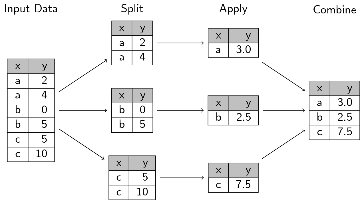
We’re taking a quick detour to briefly talk about a concept that perfectly illustrates how vectorization and functionals fit into doing data analysis. The concept is called the split-apply-combine technique, which we covered in the beginner R workshop. The method is:

Split the data into groups (e.g. diabetes status).
Apply some analysis or statistics to each group (e.g. finding the mean of age).
Combine the results to present them together (e.g. into a data frame that you can use to make a plot or table).

So when you split data into multiple groups, you create a list (or a vector) that you can then apply (e.g. with the map functional) a statistical technique to each group through vectorization, and where you finally combine (e.g. with join that we will cover later or with list_rbind()). This technique works really well for a range of tasks, including for our task of summarizing some of the DIME data so we can merge it all into one dataset.

A diagram showing how a data frame is split up, an action is applied to the splits that outputs a new result, and the results are combined back together. Taken from Software Carpentries R for Reproducible Scientific Analysis.

Functionals and vectorization are integral components of how R works and they appear throughout many of R’s functions and packages. They are particularly used throughout the tidyverse packages like dplyr. Let’s get into some more advanced features of dplyr functions that work as functionals.

There are many “verbs” in dplyr, like select(), rename(), mutate(), summarise(), and group_by() (covered in more detail in the introductory workshop). The common usage of these verbs is through acting on and directly using the column names (e.g. without " quotes around the column name). Like most tidyverse functions, dplyr verbs are designed with a strong functional programming approach. But many dplyr verbs can also be used as functionals like we covered in previous sessions with map(), where they take functions as input. For instance, summarise() uses several functional programming concepts: Create a new column using an action that may or may not be based on other columns and output a single value from that action. Using an example with our DIME data, to calculate the mean of a column and create a new column from that mean for the glucose values, you would do:

cgm_data |>
  summarise(mean_glucose = mean(historic_glucose_mmol_l))

# A tibble: 1 × 1
  mean_glucose
         <dbl>
1         5.63

This is functional in the mean() works on the vector of glucose values, so it is vectorised. This output gets added as a new column to the data frame, without you having to be explicit about how it does it. The fun parts of learning about functionals is if you wanted to calculate the mean and maybe another statistic, like the standard deviation. The “simplest” would be to do something like:

cgm_data |>
  summarise(
    mean_glucose = mean(historic_glucose_mmol_l),
    sd_glucose = sd(historic_glucose_mmol_l)
  )

# A tibble: 1 × 2
  mean_glucose sd_glucose
         <dbl>      <dbl>
1         5.63       1.13

What if you wanted to calculate the mean, standard deviation, maybe the median, and finally the maximum and minimum values? And what if you wanted to this for several different columns? That’s where the function across() comes in, which works a bit like map() does. You give it a vector of columns to work on and a list of functions to apply to those columns.

Unlike map(), which is a more general function, across() is specifically designed to work within dplyr verbs like mutate() or summarise() and within the context of a data frame.

Sticky/hat up!

When you’re ready to continue, place the sticky/paper hat on your computer to indicate this to the teacher 👒 🎩

10.3 Summarising with `across()`

🧑‍🏫 Teacher note

Open up ?across in the Console and go over the arguments with the learners. Go over the first two arguments again, reinforcing what they read.

Also, before coding again, remind everyone that we still only import the first 100 rows of each data file. So if some of the data itself seems weird, that is the reason why. Remind them that we do this to more quickly prototype and test code out.

Before we start using across(), let’s look at the help page for it. In the Console, type ?across and hit enter. This will open the help page for across(). For this workshop, we will only go over the first two arguments. The first argument is the columns you want to work on. You can use c() to combine multiple columns together. The second argument is the function you want to apply to those columns. You can use list() to combine multiple functions together.

Let’s try out using across() on the cgm_data. But before we do that, go to the setup code chunk at the top of docs/learning.qmd and let’s fix the glucose column. It’s a bit long to use, it would be nicer if it was shorter. We will use rename() like we’ve done before.

docs/learning.qmd

cgm_data <- here("data-raw/dime/cgm") |>
  import_csv_files() |>
  get_participant_id() |>
  prepare_dates(device_timestamp) |>
  rename(glucose = historic_glucose_mmol_l)

Run all the code in the setup code chunk by using Ctrl-Enter on all the lines. Then, go to the end of docs/learning.qmd, make a new header called ## Summarising with across() and create a code chunk below that with Ctrl-Alt-I or with the Palette (Ctrl-Shift-P, then type “new chunk”). For now, we will do a very simple example of using across() to calculate the mean of all the glucose values.

docs/learning.qmd

cgm_data |>
  summarise(across(glucose, mean))

# A tibble: 1 × 1
  glucose
    <dbl>
1    5.63

This is nice, but let’s try also calculating the median. The help documentation of across() says that you have to wrap multiple functions into a list(). Let’s try that:

docs/learning.qmd

cgm_data |>
  summarise(across(glucose, list(mean, median)))

# A tibble: 1 × 2
  glucose_1 glucose_2
      <dbl>     <dbl>
1      5.63       5.5

It works, but, the column names are a bit vague. The column names are glucose_1 and glucose_2, which doesn’t tell us which is which. We can add the names of the functions by using a named list. In our case, a named list would look like:

Console

list(mean = mean)

$mean
function (x, ...) 
UseMethod("mean")
<bytecode: 0x56544f0dafc0>
<environment: namespace:base>

# or
list(average = mean)

$average
function (x, ...) 
UseMethod("mean")
<bytecode: 0x56544f0dafc0>
<environment: namespace:base>

# or
list(ave = mean)

$ave
function (x, ...) 
UseMethod("mean")
<bytecode: 0x56544f0dafc0>
<environment: namespace:base>

See how the left hand side of the = is the name and the right hand side is the function? This named list is what across() can use to add the name to the end of the column name. Just like with map() we can also give it anonymous functions if our function is a bit more complex. For instance, if we needed to remove NA values from the calculations, we would do:

Console

list(mean = \(x) mean(x, na.rm = TRUE))

$mean
function (x) 
mean(x, na.rm = TRUE)

For now, we don’t need to use anonymous functions. Let’s test it with just one function, like list(mean = mean) it would look like:

docs/learning.qmd

cgm_data |>
  summarise(across(glucose, list(mean = mean)))

# A tibble: 1 × 1
  glucose_mean
         <dbl>
1         5.63

Then, we can add more functions to the named list. Let’s add the median and standard deviation:

docs/learning.qmd

cgm_data |>
  summarise(
    across(
      glucose,
      list(mean = mean, sd = sd, median = median)
    )
  )

# A tibble: 1 × 3
  glucose_mean glucose_sd glucose_median
         <dbl>      <dbl>          <dbl>
1         5.63       1.13            5.5

The great thing about using across() is that you can also use it with all the tidyselect functions in the first argument. For instance, if you wanted to only calculate things for columns that are numbers, you can use where(is.numeric) to select all the numeric columns. Or if you had a pattern in your column names, you can use things like starts_with() or ends_with() to select columns that start or end with a certain string.

Summarising works best with grouping though! Which is what we’d like to do in order to effectively join the data.

10.4 Summarising by groups

Our two datasets, the cgm_data and sleep_data, have a few columns that we’d like to join by, but the data itself can’t be joined effectively yet. We need to first summarise the data by the columns we want to join by. In the case of the cgm_data, we want to join by the id, date, and hour.

In this case, we need to use the split-apply-combined technique by first using group_by() on these variables before summarising. Let’s start with using group_by() on the cgm_data. At the bottom of the docs/learning.qmd file, create a new header called ## Summarising by groups and create a code chunk below that with Ctrl-Alt-I or with the Palette (Ctrl-Shift-P, then type “new chunk”). Then we’ll use group_by() on it’s own. But first, since we won’t be using the device_timestamp column, let’s remove it.

docs/learning.qmd

cgm_data |>
  select(-device_timestamp)

# A tibble: 1,900 × 4
      id date        hour glucose
   <int> <date>     <int>   <dbl>
 1   101 2021-03-18     8     5.8
 2   101 2021-03-18     8     5.4
 3   101 2021-03-18     8     5.1
 4   101 2021-03-18     9     5.3
 5   101 2021-03-18     9     5.3
 6   101 2021-03-18     9     4.9
 7   101 2021-03-18     9     4.7
 8   101 2021-03-18    10     4.8
 9   101 2021-03-18    10     5.5
10   101 2021-03-18    10     5.7
# ℹ 1,890 more rows

Then, let’s continue and pipe |> to group_by() for the id, date, and hour columns.

docs/learning.qmd

cgm_data |>
  select(-device_timestamp) |>
  group_by(id, date, hour)

# A tibble: 1,900 × 4
      id date        hour glucose
   <int> <date>     <int>   <dbl>
 1   101 2021-03-18     8     5.8
 2   101 2021-03-18     8     5.4
 3   101 2021-03-18     8     5.1
 4   101 2021-03-18     9     5.3
 5   101 2021-03-18     9     5.3
 6   101 2021-03-18     9     4.9
 7   101 2021-03-18     9     4.7
 8   101 2021-03-18    10     4.8
 9   101 2021-03-18    10     5.5
10   101 2021-03-18    10     5.7
# ℹ 1,890 more rows

Notice how it doesn’t do anything different? That’s because group_by() only modifies the behaviour of later functions but on it’s own doesn’t do anything. Let’s now pipe into summarise() and use across() to calculate the mean and standard deviation of the glucose values.

docs/learning.qmd

cgm_data |>
  select(-device_timestamp) |>
  group_by(id, date, hour) |>
  summarise(across(glucose, list(mean = mean, sd = sd)))

`summarise()` has grouped output by 'id', 'date'. You can override
using the `.groups` argument.

# A tibble: 506 × 5
      id date        hour glucose_mean glucose_sd
   <int> <date>     <int>        <dbl>      <dbl>
 1   101 2021-03-18     8         5.43     0.351 
 2   101 2021-03-18     9         5.05     0.300 
 3   101 2021-03-18    10         5.3      0.392 
 4   101 2021-03-18    11         4.03     0.189 
 5   101 2021-03-18    12         4.02     0.0957
 6   101 2021-03-18    13         4.1      0.141 
 7   101 2021-03-18    14         5.62     0.946 
 8   101 2021-03-18    15         7.3      0.141 
 9   101 2021-03-18    16         6.55     0.7   
10   101 2021-03-18    17         4.8      0.356 
# ℹ 496 more rows

Very neat! By default, when we use group_by() it continues to tell R to use dplyr functions on the groups, for instance with mutate() and summarise(). Often we want to only do a single action on groups, so we would need to stop grouping by using ungroup(). This is especially a common practice when you use group_by() with summarise(). That’s why summarise() has an argument to drop the grouping with .groups = "drop" rather than have to pipe to ungroup(). We don’t need to group any more, so we will add this:

docs/learning.qmd

cgm_data |>
  select(-device_timestamp) |>
  group_by(id, date, hour) |>
  summarise(
    across(
      glucose,
      list(mean = mean, sd = sd)
    ),
    .groups = "drop"
  )

# A tibble: 506 × 5
      id date        hour glucose_mean glucose_sd
   <int> <date>     <int>        <dbl>      <dbl>
 1   101 2021-03-18     8         5.43     0.351 
 2   101 2021-03-18     9         5.05     0.300 
 3   101 2021-03-18    10         5.3      0.392 
 4   101 2021-03-18    11         4.03     0.189 
 5   101 2021-03-18    12         4.02     0.0957
 6   101 2021-03-18    13         4.1      0.141 
 7   101 2021-03-18    14         5.62     0.946 
 8   101 2021-03-18    15         7.3      0.141 
 9   101 2021-03-18    16         6.55     0.7   
10   101 2021-03-18    17         4.8      0.356 
# ℹ 496 more rows

Ungrouping the data with the .groups = "drop" in the summarise() function does not do anything except to tell R not to do any more grouping when you use later functions.

This workflow is very similar to how we want to do it with the sleep_data. And as you can guess, we’ll need to make a function. However! There’s a few things things we could do now to simplify making the function.

The sleep data has an extra sleep_type column that we have to group by. We’d rather not have to include an argument in our new function just for indicating the grouping. It would be nice if we could group by all columns except for the column we want to summarise.
We don’t really want to group by device_timestamp or datetime columns. It would be nice if we could exclude those columns from the grouping in a way that can be used for both datasets without having an error.

For the second, we can use some tidyselect functions like contains() with a - to exclude the columns. For the first, there’s a handy function in the dplyr package called pick(). This function lets us use tidyselect functions to include or exclude columns. Let’s start with the contains() function. Let’s write it so it will drop any column that has the name of either device_timestamp or datetime from the dataset. Revise the select() function we’ve already written and use contains():

docs/learning.qmd

cgm_data |>
  select(-contains("timestamp"), -contains("datetime")) |>
  group_by(id, date, hour) |>
  summarise(
    across(
      glucose,
      list(mean = mean, sd = sd)
    ),
    .groups = "drop"
  )

# A tibble: 506 × 5
      id date        hour glucose_mean glucose_sd
   <int> <date>     <int>        <dbl>      <dbl>
 1   101 2021-03-18     8         5.43     0.351 
 2   101 2021-03-18     9         5.05     0.300 
 3   101 2021-03-18    10         5.3      0.392 
 4   101 2021-03-18    11         4.03     0.189 
 5   101 2021-03-18    12         4.02     0.0957
 6   101 2021-03-18    13         4.1      0.141 
 7   101 2021-03-18    14         5.62     0.946 
 8   101 2021-03-18    15         7.3      0.141 
 9   101 2021-03-18    16         6.55     0.7   
10   101 2021-03-18    17         4.8      0.356 
# ℹ 496 more rows

When we run this with Ctrl-Enter it works, even though datetime doesn’t exist. That’s because contains() only gets the column if is there and if it isn’t there, it doesn’t do anything. Now, let’s try using pick(). In this case, we can use -glucose to exclude the glucose column:

docs/learning.qmd

cgm_data |>
  select(-contains("timestamp"), -contains("datetime")) |>
  group_by(pick(-glucose)) |>
  summarise(
    across(
      glucose,
      list(mean = mean, sd = sd)
    ),
    .groups = "drop"
  )

# A tibble: 506 × 5
      id date        hour glucose_mean glucose_sd
   <int> <date>     <int>        <dbl>      <dbl>
 1   101 2021-03-18     8         5.43     0.351 
 2   101 2021-03-18     9         5.05     0.300 
 3   101 2021-03-18    10         5.3      0.392 
 4   101 2021-03-18    11         4.03     0.189 
 5   101 2021-03-18    12         4.02     0.0957
 6   101 2021-03-18    13         4.1      0.141 
 7   101 2021-03-18    14         5.62     0.946 
 8   101 2021-03-18    15         7.3      0.141 
 9   101 2021-03-18    16         6.55     0.7   
10   101 2021-03-18    17         4.8      0.356 
# ℹ 496 more rows

Let’s run it with Ctrl-Enter and see that it works. Woohoo! 🎉 Now it’s time to make it a function 😁 Well, almost. We’ve so far been creating functions that prepare the datasets and then piping those functions together after importing the data into the setup code chunk. That’s fine, but maybe a bit tedious. It would be nice if we had two functions called clean_cgm() and clean_sleep() that we could use to pipe from import_csv_files(). And that any new cleaning function we create we can just put into those cleaning functions.

So, let’s do that. First, go to the setup code chunk and cut the cleaning code for CGM data. Then open up the R/functions.R file, either manually or with Ctrl-.. Scroll to the bottom of the file and create a new clean_cgm() function. During the exercise you will create the clean_sleep() function. Paste the code into this new function:

#' Clean and prepare the CGM data for joining.
#'
#' @param data The CGM dataset.
#'
#' @returns A cleaner data frame.
#'
clean_cgm <- function(data) {
  cleaned <- data |>
    get_participant_id() |>
    prepare_dates(device_timestamp) |>
    dplyr::rename(glucose = historic_glucose_mmol_l)
  return(cleaned)
}

Then, in the setup code chunk of docs/learning.qmd, replace the cut code with:

docs/learning.qmd

cgm_data <- here("data-raw/dime/cgm") |>
  import_csv_files() |>
  clean_cgm()

Amazing! Before continuing to the exercise, let’s run styler with the Palette (Ctrl-Shift-P, then type “style file”) on both docs/learning.qmd and on R/functions.R. Then we will render the Quarto document with Ctrl-Shift-K or with the Palette (Ctrl-Shift-P, then type “render”) to confirm that everything runs as it should. If the rendering works, switch to the Git interface and add and commit the changes so far with Ctrl-Alt-M or with the Palette (Ctrl-Shift-P, then type “commit”) and push to GitHub.

10.5 Converting the summarising code into a function

Let’s start with converting the summarising code into a function. First, we’ll assign function() to a new named function called summarise_column and include three arguments in function() with the names data, column, and functions.

Then we’ll put the code we just wrote into the body of the function. Make sure to return() the output at the end of the function. Replace the relevant variables with the arguments you just created (e.g. cgm_data to data). As we learned about the {{ }}, we’ll wrap it around the column argument within the function. That way the function will work with tidyverse’s and R’s non-standard evaluation.

We’ll then add the Roxygen documentation with Ctrl-Shift-Alt-R or with the Palette (Ctrl-Shift-P, then type “roxygen comment”) and fill it out.

Then we’ll explicitly link the functions you are using in this new function to their package by using :: (e.g. dplyr:: and tidyselect::).

#' Summarise a single column based on one or more functions.
#'
#' @param data Either the CGM or sleep data in DIME.
#' @param column The name of the column you want to summarise.
#' @param functions One or more functions to apply to the column. If more than
#'    one, use `list()`.
#'
#' @returns A summarised data frame.
#'
summarise_column <- function(data, column, functions) {
  summarised <- data |>
    dplyr::select(
      -tidyselect::contains("timestamp"),
      -tidyselect::contains("datetime")
    ) |>
    dplyr::group_by(dplyr::pick(-{{ column }})) |>
    dplyr::summarise(
      dplyr::across(
        {{ column }},
        functions
      ),
      .groups = "drop"
    )
  return(summarised)
}

Since we’re using tidyselect, we’ll need to add that as a dependency:

Console

usethis::use_package("tidyselect")

Test that the function works by using the code shown above.

cgm_data |>
  summarise_column(glucose, list(mean = mean, sd = sd))

# A tibble: 506 × 5
      id date        hour glucose_mean glucose_sd
   <int> <date>     <int>        <dbl>      <dbl>
 1   101 2021-03-18     8         5.43     0.351 
 2   101 2021-03-18     9         5.05     0.300 
 3   101 2021-03-18    10         5.3      0.392 
 4   101 2021-03-18    11         4.03     0.189 
 5   101 2021-03-18    12         4.02     0.0957
 6   101 2021-03-18    13         4.1      0.141 
 7   101 2021-03-18    14         5.62     0.946 
 8   101 2021-03-18    15         7.3      0.141 
 9   101 2021-03-18    16         6.55     0.7   
10   101 2021-03-18    17         4.8      0.356 
# ℹ 496 more rows

sleep_data |>
  summarise_column(seconds, sum)

# A tibble: 1,258 × 5
      id date        hour sleep_type seconds
   <int> <date>     <int> <chr>        <dbl>
 1   101 2021-05-21    23 deep           390
 2   101 2021-05-21    23 light         2730
 3   101 2021-05-21    23 wake           450
 4   101 2021-05-22     0 deep          1200
 5   101 2021-05-22     0 light         1230
 6   101 2021-05-22     0 rem           1620
 7   101 2021-05-22     1 deep           420
 8   101 2021-05-22     1 light         2970
 9   101 2021-05-22     2 light         3870
10   101 2021-05-22     2 rem           1050
# ℹ 1,248 more rows

After we’ve created the function and tested it, move (cut and paste) the function into R/functions.R. In the next exercise, you will use this function in the recently created clean_cgm() and the clean_sleep() function you will create.

10.6 🧑‍💻 Exercise: Create a `clean_sleep()` function

Time: ~15 minutes.

Just like we did with the clean_cgm() function, you will create a a clean_sleep() function here that will contain the functions you’ve made to clean it up. You also now have the summarise_column() function, that you can include in both the clean_cgm() and clean_sleep() functions. In the end, the code should look like this in the setup code chunk:

docs/learning.qmd

cgm_data <- here("data-raw/dime/cgm") |>
  import_csv_files() |>
  clean_cgm()
sleep_data <- here("data-raw/dime/sleep") |>
  import_csv_files() |>
  clean_sleep()

And if you were to run these in the Console, it might look like:

Console

cgm_data

# A tibble: 506 × 5
      id date        hour glucose_mean glucose_sd
   <int> <date>     <int>        <dbl>      <dbl>
 1   101 2021-03-18     8         5.43     0.351 
 2   101 2021-03-18     9         5.05     0.300 
 3   101 2021-03-18    10         5.3      0.392 
 4   101 2021-03-18    11         4.03     0.189 
 5   101 2021-03-18    12         4.02     0.0957
 6   101 2021-03-18    13         4.1      0.141 
 7   101 2021-03-18    14         5.62     0.946 
 8   101 2021-03-18    15         7.3      0.141 
 9   101 2021-03-18    16         6.55     0.7   
10   101 2021-03-18    17         4.8      0.356 
# ℹ 496 more rows

sleep_data

# A tibble: 1,258 × 5
      id date        hour sleep_type seconds_sum
   <int> <date>     <int> <chr>            <dbl>
 1   101 2021-05-21    23 deep               390
 2   101 2021-05-21    23 light             2730
 3   101 2021-05-21    23 wake               450
 4   101 2021-05-22     0 deep              1200
 5   101 2021-05-22     0 light             1230
 6   101 2021-05-22     0 rem               1620
 7   101 2021-05-22     1 deep               420
 8   101 2021-05-22     1 light             2970
 9   101 2021-05-22     2 light             3870
10   101 2021-05-22     2 rem               1050
# ℹ 1,248 more rows

To get to this point, do the following tasks:

Go to the setup code chunk in your docs/learning.qmd file and cut the code that cleans the sleep data. Cut the code that is piped after using import_csv_files() but don’t cut the import_csv_files() line.
Then, open up the R/functions.R file and create a new function called clean_sleep, that has the same argument as clean_cgm() (data).
Paste the cleaning code you just cut into this new function.
Put data at the top of the code and pipe it into the cleaning code.
At the end of the cleaning pipe, continue with a pipe into summarise_column(). Use the seconds column and the sum() function (you can use either list(sum = sum) or just simply sum in summarise_column()). Why sum? Because the average seconds doesn’t make sense here, we want the total time slept in each stage. This will calculate the time slept each hour in each stage for each night, by each participant.
Assign the output of the cleaning code to a new variable called cleaned, like we did with clean_cgm().
Include a return() statement at the end of the function to return the cleaned data.
Create some Roxygen documentation of the function with Ctrl-Shift-Alt-R or with the Palette (Ctrl-Shift-P, then type “roxygen comment”).
Before using the new clean_sleep() function, go to the clean_cgm() function and add the summarise_column() function to the end of the pipe inside the clean_cgm() function. Use the glucose column and decide on which functions you want to summarise by, e.g. list(mean = mean, sd = sd) or maybe instead of mean, use the median.
Go to your docs/learning.qmd file and in the setup code chunk, pipe the output of import_csv_files(here("data-raw/dime/sleep/")) into the new clean_sleep() function.
Run styler in both the R/functions.R file and docs/learning.qmd with the Palette (Ctrl-Shift-P, then type “style file”).
Render the Quarto document with Ctrl-Shift-K or with the Palette (Ctrl-Shift-P, then type “render”) to confirm that everything runs as it should.
Add and commit the changes to the Git history with Ctrl-Alt-M or with the Palette (Ctrl-Shift-P, then type “commit”). Then push to GitHub.

Sticky/hat up!

When you’re ready to continue, place the sticky/paper hat on your computer to indicate this to the teacher 👒 🎩

10.7 Key takeaways

Teacher note

Quickly cover this and get them to do the survey before moving on to the discussion activity.

The split-apply-combine technique is a powerful way to summarise and analyse data in R. It allows you to split your data into groups, apply a function to each group, and then combine the results back together. Re-framing how you think about your data using this technique can substantially help you in your data analysis.
Use group_by(), summarise(), and across() with .groups = "drop" in the summarise() function to use the split-apply-combine technique when needing to do an action on groups within the data (e.g. calculate the mean age between education groups).
Build functions to be able to chain together and then convert those chained functions into general functions. That way you can create more “higher-level” functions to help keep your code organised, readable, and maintainable.

10.8 💬 Discussion activity: How might you split-apply-combine in your work?

Time: ~6 minutes.

As we prepare for the next session and taking a break, get up and discuss with your neighbour (or others) the questions:

From what you have learned so far from this session, how might you use this in your work?
Can you consider how these functions and approaches can simplify or shorten code you use to do your analyses?
Are there other ways you can use this other than with your research data? For instance, organising courses?

10.9 Code used in session

This lists some, but not all, of the code used in the section. Some code is incorporated into Markdown content, so is harder to automatically list here in a code chunk. The code below also includes the code from the exercises.

cgm_data <- here("data-raw/dime/cgm") |>
  import_csv_files() |>
  get_participant_id() |>
  prepare_dates(device_timestamp) |>
  rename(glucose = historic_glucose_mmol_l)
cgm_data |>
  summarise(across(glucose, mean))
cgm_data |>
  summarise(across(glucose, list(mean, median)))
list(mean = mean)
# or
list(average = mean)
# or
list(ave = mean)
list(mean = \(x) mean(x, na.rm = TRUE))
cgm_data |>
  summarise(across(glucose, list(mean = mean)))
cgm_data |>
  summarise(
    across(
      glucose,
      list(mean = mean, sd = sd, median = median)
    )
  )
cgm_data |>
  select(-device_timestamp)
cgm_data |>
  select(-device_timestamp) |>
  group_by(id, date, hour)
cgm_data |>
  select(-device_timestamp) |>
  group_by(id, date, hour) |>
  summarise(across(glucose, list(mean = mean, sd = sd)))
cgm_data |>
  select(-device_timestamp) |>
  group_by(id, date, hour) |>
  summarise(
    across(
      glucose,
      list(mean = mean, sd = sd)
    ),
    .groups = "drop"
  )
cgm_data |>
  select(-contains("timestamp"), -contains("datetime")) |>
  group_by(id, date, hour) |>
  summarise(
    across(
      glucose,
      list(mean = mean, sd = sd)
    ),
    .groups = "drop"
  )
cgm_data |>
  select(-contains("timestamp"), -contains("datetime")) |>
  group_by(pick(-glucose)) |>
  summarise(
    across(
      glucose,
      list(mean = mean, sd = sd)
    ),
    .groups = "drop"
  )
#' Clean and prepare the CGM data for joining.
#'
#' @param data The CGM dataset.
#'
#' @returns A cleaner data frame.
#'
clean_cgm <- function(data) {
  cleaned <- data |>
    get_participant_id() |>
    prepare_dates(device_timestamp) |>
    dplyr::rename(glucose = historic_glucose_mmol_l)
  return(cleaned)
}
cgm_data <- here("data-raw/dime/cgm") |>
  import_csv_files() |>
  clean_cgm()
#' Summarise a single column based on one or more functions.
#'
#' @param data Either the CGM or sleep data in DIME.
#' @param column The name of the column you want to summarise.
#' @param functions One or more functions to apply to the column. If more than
#'    one, use `list()`.
#'
#' @returns A summarised data frame.
#'
summarise_column <- function(data, column, functions) {
  summarised <- data |>
    dplyr::select(
      -tidyselect::contains("timestamp"),
      -tidyselect::contains("datetime")
    ) |>
    dplyr::group_by(dplyr::pick(-{{ column }})) |>
    dplyr::summarise(
      dplyr::across(
        {{ column }},
        functions
      ),
      .groups = "drop"
    )
  return(summarised)
}
usethis::use_package("tidyselect")
#' Clean and prepare the sleep data for joining.
#'
#' @param data The sleep dataset.
#'
#' @returns A cleaner data frame.
#'
clean_sleep <- function(data) {
  cleaned <- data |>
    get_participant_id() |>
    dplyr::rename(datetime = date) |>
    prepare_dates(datetime) |>
    summarise_column(seconds, list(sum = sum))
  return(cleaned)
}
#' Clean and prepare the CGM data for joining.
#'
#' @param data The CGM dataset.
#'
#' @returns A cleaner data frame.
#'
clean_cgm <- function(data) {
  cleaned <- data |>
    get_participant_id() |>
    prepare_dates(device_timestamp) |>
    dplyr::rename(glucose = historic_glucose_mmol_l) |>
    # You can decide what functions to summarise by.
    summarise_column(glucose, list(mean = mean, sd = sd))
  return(cleaned)
}