Click for the solution. Only click if you are struggling or are out of time.
"user_[1-9][0-9]?"🚧 We are doing major changes to this workshop, so much of the content will be changed. 🚧
Describe some ways to join or “bind” data and identify which join is appropriate for a given situation. Then apply dplyr’s full_join() function to join two datasets together into one single dataset.
Demonstrate how to use functionals to repeatedly join more than two datasets together.
Apply the function case_when() in situations that require nested conditionals (if-else).
Before we go into joining datasets together, we have to do a bit of processing first. Specifically, we want to get the user ID from the file_path_id character data. Whenever you are processing and cleaning data, you will very likely encounter and deal with character data. A wonderful package to use for working with character data is called stringr, which we’ll use to extract the user ID from the file_path_id column.
The main driver behind the functions in stringr are regular expressions (or regex for short). These expressions are powerful, very concise ways of finding patterns in text. Because they are so concise, though, they are also very very difficult to learn, write, and read, even for experienced users. That’s because certain characters like [ or ? have special meanings. For instance, [aeiou] is regex for “find one character in a string that is either a, e, i, o, or u”. The [] in this case mean “find the character in between the two brackets”. We won’t cover regex too much in this workshop, some great resources for learning them are the R for Data Science regex section, the stringr regex page, as well as in the help doc ?regex.
We’ve already used them a bit in the dir_ls() function with the regexp argument to find our data files. In the case of the regex in our use of dir_ls(), we had wanted to find, for instance, the pattern "user_info.csv" in all the folders and files. But in this case, we want to extract the user ID pattern, from user_1 to user_22. So how would we go about extracting this pattern?
Time: 10 minutes.
In your groups do these tasks. Try not to look ahead, nor in the solution section 😉! When the time is up, we’ll share some ideas and go over what the regex will be.
file_path_id column, list what is similar in the user ID between rows and what is different.user will find only user.[] to find one possible character of the several between the brackets. E.g. [12] means 1 or 2 or [ab] means “a” or “b”. To find a range of numbers or letters, use - in between the start and end ranges, e.g. [1-3] means 1 to 3 or [a-c] means “a” to “c”.? if the character might be there or not. E.g. ab? means “a” and maybe “b” follows it or 1[1-2]? means 1 and maybe 1 or 2 will follow it.Once you’ve done these tasks, we’ll discuss all together and go over what the regex would be to extract the user ID.
"user_[1-9][0-9]?"Now that we’ve identified a possible regex to use to extract the user ID, let’s test it out on the user_info_df data. Once it works, we will convert it into a function and move (cut and paste) it into the R/functions.R file.
Since we will create a new column for the user ID, we will use the mutate() function from the dplyr package. We’ll use the str_extract() function from the stringr package to “extract a string” by using the regex user_[1-9][0-9]? that we discussed from the exercise. Since we’re going to use stringr, so let’s add it as a package dependency by typing this in the Console:
Console
usethis::use_package("stringr")We’re also using an argument to mutate() you might not have seen previously, called .before. This will insert the new user_id column before the column we use and we do this entirely for visual reasons, since it is easier to see the newly created column when we run the code. In your docs/learning.qmd file, create a new header called ## Using regex for user ID at the bottom of the document, and create a new code chunk below that.
docs/learning.qmd
user_info_df <- import_multiple_files("user_info.csv", import_user_info)
# Note: your file paths and data may look slightly different.
user_info_df |>
  mutate(
    user_id = str_extract(
      file_path_id,
      "user_[1-9][0-9]?"
    ),
    .before = file_path_id
  )
Since we don’t need the file_path_id column anymore, let’s drop it using select() and -.
docs/learning.qmd
user_info_df |>
  mutate(
    user_id = str_extract(
      file_path_id,
      "user_[1-9][0-9]?"
    ),
    .before = file_path_id
  ) |>
select(-file_path_id)Time: 15 minutes.
We now have code that takes the data that has the file_path_id column and extracts the user ID from it. First step: While in the docs/learning.qmd file, convert this code into a function, using the same process you’ve done previously.
Use this code as a guide to help complete the exercise tasks below:
docs/learning.qmd
extract_user_id <- ___(___) {
    ___ <- ___ |>
        ___mutate(
            user_id = ___str_extract(file_path_id,
                                     "user_[0-9][0-9]?"),
            .before = file_path_id
        ) |>
        ___select(-file_path_id)
    return(___)
}

# This tests that it works:
# extract_user_id(user_info_df)extract_user_id and add one argument called imported_data.
return() it at the end of the function.R/functions.R.R/functions.R file with the Palette (Ctrl-Shift-PCtrl-Shift-P, then type “style file”).docs/learning.qmd file with the function name so it looks like extract_user_id(user_info_df), restart the R session, source everything with source() with Ctrl-Shift-SCtrl-Shift-S or with the Palette (Ctrl-Shift-PCtrl-Shift-P, then type “source”), and run the new function in the code chunk inside the docs/learning.qmd to test that it works. This should automatically run the setup code chunk, otherwise, run that chunk if it doesn’t.docs/learning.qmd file to make sure things remain reproducible with Ctrl-Shift-KCtrl-Shift-K or with the Palette (Ctrl-Shift-PCtrl-Shift-P, then type “render”).#' Extract user ID from data with file path column.
#'
#' @param imported_data Data with `file_path_id` column.
#'
#' @return A data.frame/tibble.
#'
extract_user_id <- function(imported_data) {
extracted_id <- imported_data |>
dplyr::mutate(
user_id = stringr::str_extract(
file_path_id,
"user_[0-9][0-9]?"
),
.before = file_path_id
) |>
dplyr::select(-file_path_id)
return(extracted_id)
}
# This tests that it works:
extract_user_id(user_info_df)Now that we’ve created a new function to extract the user ID from the file path variable, we need to actually use it within our processing pipeline. Since we want this function to work on all the datasets that we will import, we need to add it to the import_multiple_files() function. We’ll go to the import_multiple_files() function in R/functions.R and use the |> to add it after using the list_rbind() function. The code should look something like:
R/functions.R
import_multiple_files <- function(file_pattern, import_function) {
  data_files <- fs::dir_ls(here::here("data-raw/mmash/"),
    regexp = file_pattern,
    recurse = TRUE
  )

  combined_data <- purrr::map(data_files, import_function) |>
    purrr::list_rbind(names_to = "file_path_id") |>
    extract_user_id() # Add the function here
  return(combined_data)
}
We’ll re-source the functions with source() using Ctrl-Shift-SCtrl-Shift-S or with the Palette (Ctrl-Shift-PCtrl-Shift-P, then type “source”). Then re-run these pieces of code you wrote during the exercise in Section 8.3 to update them based on the new code in the import_multiple_files() function. Add this to your docs/learning.qmd file for now.
docs/learning.qmd
user_info_df <- import_multiple_files("user_info.csv", import_user_info)
saliva_df <- import_multiple_files("saliva.csv", import_saliva)
rr_df <- import_multiple_files("RR.csv", import_rr)
actigraph_df <- import_multiple_files("Actigraph.csv", import_actigraph)
As well as adding the summarised_rr_df and summarised_actigraph_df to use user_id instead of file_path_id:
docs/learning.qmd
summarised_rr_df <- rr_df |>
  group_by(user_id, day) |> # change file_path_id to user_id here
  summarise(
    across(ibi_s, list(
      mean = \(x) mean(x, na.rm = TRUE),
      sd = \(x) sd(x, na.rm = TRUE)
    )),
    .groups = "drop"
  )

summarised_actigraph_df <- actigraph_df |>
  group_by(user_id, day) |> # change file_path_id to user_id here
  # These statistics will probably be different for you
  summarise(
    across(hr, list(
      mean = \(x) mean(x, na.rm = TRUE),
      sd = \(x) sd(x, na.rm = TRUE)
    )),
    .groups = "drop"
  )
Let’s render the docs/learning.qmd document using Ctrl-Shift-KCtrl-Shift-K or with the Palette (Ctrl-Shift-PCtrl-Shift-P, then type “render”) to make sure everything still runs fine. Then, add and commit all the changed files into the Git history with Ctrl-Alt-MCtrl-Alt-M or with the Palette (Ctrl-Shift-PCtrl-Shift-P, then type “commit”).
The ability to join datasets together is a fundamental component of data processing and transformation. In our case, we want to add the datasets together so we eventually have preferably one main dataset to work with.
There are many ways to join datasets in dplyr that are described in ?dplyr::join. The more common ones that are implemented in the dplyr package are:
left_join(x, y): Join all rows and columns in y that match rows and columns in x. Columns that exist in y but not x are joined to x.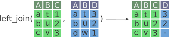
d in column A) is not included in the outputted data on the right. Modified from the Posit dplyr cheat sheet.
right_join(x, y): The opposite of left_join(). Join all rows and columns in x that match rows and columns in y. Columns that exist in x but not y are joined to y.
c in column A) is not included in the outputted data on the right. Modified from the Posit dplyr cheat sheet.
full_join(x, y): Join all rows and columns in y that match rows and columns in x. Columns and rows that exist in y but not x are joined to x. A full join keeps all the data from both x and y.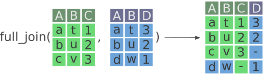
Now, we want to start joining our datasets. Let’s start with the user_info_df and saliva_df. In this case, we want to use full_join(), since we want all the data from both datasets. This function takes two datasets and lets you indicate which column to join by using the by argument. Here, both datasets have the column user_id so we will join by that column.
full_join(user_info_df, saliva_df, by = "user_id")full_join() is useful if we want to include all values from both datasets, as long as each participant (“user”) had data collected from either dataset. When the two datasets have rows that don’t match, we will get missingness in that row, but that’s ok in this case.
We also eventually have other datasets to join together later on. Since full_join() can only take two datasets at a time, do we then just keep using full_join() until all the other datasets are combined? What if we get more data later on? Well, that’s where more functional programming comes in. Again, we have a simple goal: For a set of data frames, join them all together. Here we use another functional programming concept from the purrr package called reduce(). Like map(), which “maps” a function onto a set of items, reduce() applies a function to each item of a vector or list, each time reducing the set of items down until only one remains: the output. Let’s use an example with our simple function add_numbers() we had created earlier on and add up 1 to 5. Since add_numbers() only takes two numbers, we have to give it two numbers at a time and repeat until we reach 5.
# Add from 1 to 5
first <- add_numbers(1, 2)
second <- add_numbers(first, 3)
third <- add_numbers(second, 4)
add_numbers(third, 5)
Instead, we can use reduce to do the same thing:
reduce(1:5, add_numbers)Figure 10.4 visually shows what is happening within reduce().
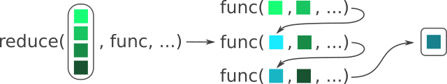
func() is placed in the first position of func() in the next iteration, and so on. Modified from the Posit purrr cheat sheet.
If we look at the documentation for reduce() by writing ?reduce in the Console, we see thatreduce(), likemap(), takes either a vector or a list as an input. Since data frames can only be put together as a list and not as a vector (a data frame has vectors for columns and so it can’t be a vector itself), we need to combine the datasets together in a list() to be able to reduce them with full_join().
Let’s code this together, using reduce(), full_join(), and list() while in the docs/learning.qmd file.
We now have the data in a form that would make sense to join it with the other datasets. So lets try it:
Hmm, but wait, we now have four rows of each user, when we should have only two, one for each day. By looking at each dataset we joined, we can find that the saliva_df doesn’t have a day column and instead has a samples column. We’ll need to add a day column in order to join properly with the RR dataset. For this, we’ll learn about using nested conditionals.
There are many ways to clean up this particular problem, but probably the easiest, most explicit, and programmatically accurate way of doing it would be with the function case_when(). This function works by providing it with a series of logical conditions and an associated output if the condition is true. Each condition is processed sequentially, meaning that if a condition is TRUE, the output won’t be overridden for later conditions. The general form of case_when() looks like:
case_when(
  variable1 == condition1 ~ output,
  variable2 == condition2 ~ output,
  # (Optional) Otherwise
  TRUE ~ final_output
)
The optional ending is only necessary if you want a certain output if none of your conditions are met. Because conditions are processed sequentially and because it is the last condition, by setting it as TRUE the final output will used. If this last TRUE condition is not used then by default, the final output would be a missing value. A (silly) example using age might be:
case_when(
  age > 20 ~ "old",
  age <= 20 ~ "young",
  # For final condition
  TRUE ~ "unborn!"
)
If instead you want one of the conditions to be NA, you need to set the appropriate NA value:
case_when(
  age > 20 ~ "old",
  age <= 20 ~ NA_character_,
  # For final condition
  TRUE ~ "unborn!"
)
Alternatively, if we want missing age values to output NA values at the end (instead of "unborn!"), we would exclude the final condition:
case_when(
  age > 20 ~ "old",
  age <= 20 ~ "young"
)
With dplyr functions like case_when(), it requires you be explicit about the type of output each condition has since all the outputs must match (e.g. all character or all numeric). This prevents you from accidentally mixing e.g. numeric output with character output. Missing values also have data types:
NA_character_ (character)NA_real_ (numeric)NA_integer_ (integer)Assuming the final output is NA, in a pipeline this would look like how you normally would use mutate():
While still in the docs/learning.qmd file, we can use the case_when() function to set "before sleep" as day 1 and "wake up" as day 2 by creating a new column called day. (We will use NA_real_ because the other day columns are numeric, not integer.)
…Now, let’s use the reduce() with full_join() again:
We now have two rows per participant! Let’s add and commit the changes to the Git history with Ctrl-Alt-MCtrl-Alt-M or with the Palette (Ctrl-Shift-PCtrl-Shift-P, then type “commit”).
Now that we’ve got several datasets processed and joined, it’s time to bring it all together so we can create a final working dataset.
We do this by saving our last, final dataset we created as dime into the data/ folder. We’ll use the function readr::write_csv() to do this, but first we need to create the folder. So at the bottom of the docs/learning.qmd file, create a header called ## Saving the final data and then make a new code chunk with ?var:keybind.r. In this code chunk, we’ll use fs::dir_create() to make the folder:
docs/learning.qmd
fs::dir_create(here("data"))Then we save it with write_csv():
And later load it in with read_csv() (since it is so fast). Alright, we’re finished creating this dataset! Let’s generate it by:
docs/learning.qmd file with Ctrl-Shift-KCtrl-Shift-K or with the Palette (Ctrl-Shift-PCtrl-Shift-P, then type “render”).We now have a final dataset to start working on! The main way to load data is with read_csv(here("data/mmash.csv")). Lastly, add and commit all the changes, including adding the final mmash.csv data file, to the Git history by using Ctrl-Alt-MCtrl-Alt-M or with the Palette (Ctrl-Shift-PCtrl-Shift-P, then type “commit”).
left_join(), right_join(), and full_join() to join two datasets together.reduce() to iteratively apply a function to a set of items in order to end up with one item (e.g. join more than two datasets into one final dataset).case_when() instead of nesting multiple “if else” conditions whenever you need to do slightly more complicated conditionals.