Want to help out or contribute?

If you find any typos, errors, or places where the text may be improved, please let us know by providing feedback either in the feedback survey (given during class) or by using GitHub.

On GitHub open an issue or submit a pull request by clicking the " Edit this page" link at the side of this page.

9  Quickly re-arranging data with pivots

Here we will continue using the Workflow block as we cover the fourth block, “Work with project data” in Figure 9.1.

Figure 9.1: Section of the overall workflow we will be covering.

Briefly go over the bigger picture (found in the introduction section) and remind everyone the ‘what’ and ‘why’ of what we are doing.

9.1 Learning objectives

  1. Using the concept of “pivoting” to arrange data from long to wide and vice versa.

9.2 Setup for the analysis in Quarto

We now have a working dataset to start doing some simple analyses on in the Quarto document. A recommended workflow with Quarto is to often render / “knit” it and make sure your analysis is reproducible (while on your computer). We already cleaned it up from the previous session.

We will now add the load() code right below the source() function in the setup code chunk:

source(here("R/functions.R"))
load(here("data/mmash.rda"))

As we write more R code and do some simple analyses of the data, we are going to be knitting fairly often (depending on how long the analysis takes of course). The main reason for this is to ensure that whatever you are writing and coding will at least be reproducible on your computer, since Quarto is designed to ensure the document is reproducible.

For this specific workflow and for checking reproducibility, you should output to HTML rather than to a Word document. While you can create a Word document by changing the format: html to format: docx (for Quarto only) at the top in the YAML header, you’d only do this when you need to submit to a journal or need to email to co-authors for review. The reason is simple: After you generate the Word document from Quarto, the Word file opens up and consequently Word locks the file from further edits. What that means is that every time you generate the Word document, you have to close it before you can generate it again, otherwise knitting / rendering will fail. This can get annoying very quickly (trust me), since you don’t always remember to close the Word document. If you output to HTML, this won’t be a problem.

9.3 Re-arranging data for easier summarizing

Let them read through this section and then walk through it again and explain it a bit more, making use of the tables and graphs. Doing both reading and listening again will help reinforce the concept of pivoting, which is usually quite difficult to grasp for those new to it.

Reading task: ~6 minutes

Now that we have the final dataset to work with, we want to explore it a bit with some simple descriptive statistics. One extremely useful and powerful tool to summarizing data is by “pivoting” your data. Pivoting is when you convert data between longer forms (more rows) and wider forms (more columns). The tidyr package within tidyverse contains two wonderful functions for pivoting: pivot_longer() and pivot_wider(). There is a well written documentation on pivoting in the tidyr website that can explain more about it. The first thing we’ll use, and probably the more commonly used in general, is pivot_longer(). This function is commonly used because entering data in the wide form is easier and more time efficient than entering data in long form. For instance, if you were measuring glucose values over time in participants, you might enter data in like this:

Example of a wide dataset that is useful for data entry.
person_id glucose_0 glucose_30 glucose_60
1 5.6 7.8 4.5
2 4.7 9.5 5.3
3 5.1 10.2 4.2

However, when it comes time to analyze the data, this wide form is very inefficient and difficult to computationally and statistically work with. So, we do data entry in wide and use functions like pivot_longer() to get the data ready for analysis. Figure 9.2 visually shows what happens when you pivot from wide to long.
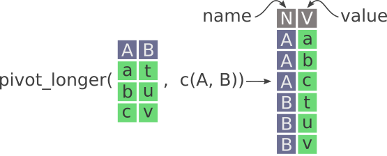
Figure 9.2: Pivot longer in tidyr. New columns are called ‘name’ and ‘value’. Notice how the values in A and B columns are stacked on top of each other in the newly created V column.

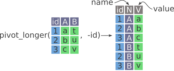
If you had, for instance, an ID column for each participant, the pivoting would look like what is shown in Figure 9.3.

Figure 9.3: Pivot longer in tidyr, excluding an ‘id’ column. New columns are called ‘name’ and ‘value’, as well as the old ‘id’ column. Notice how, unlike the previous image, the id column is excluded when pivotting into the data on the right.

Pivoting is a conceptually challenging thing to grasp, so don’t be disheartened if you can’t understand how it works yet. As you practice using it, you will understand it. With pivot_longer(), the first argument is the data itself. The other arguments are:

  1. cols: The columns to use to convert to long form. The input is a vector made using c() that contains the column names, like you would use in select() (e.g. you can use the select_helpers like starts_with(), or - minus to exclude).
  2. names_to: Optional, the default is name. If provided, it will be the name of the newly created column (as a quoted character) that contains the original column names.
  3. values_to: Optional, the default is value. Like names_to, sets the name of the new columns.

Both pivot_longer() and its opposite pivot_wider(), which we will cover later in the session, are incredibly powerful functions. We can’t show close to everything it can do in this course, but if you want to learn more, read up on the documentation for it.

Since we’ll be using tidyr, we will need to add it as a dependency by running this in the Console:

usethis::use_package("tidyr")

Let’s try this out with mmash. In your doc/learning.qmd file, create a new header called ## Pivot longer and create a new code chunk below that with linux=Ctrl-Alt-I or with the Palette (linux=Ctrl-Shift-P, then type “new chunk”). Now we can start typing in our code:

mmash |>
  # pivot every column
  pivot_longer(everything())
#> Error in `pivot_longer()`:
#> ! Can't combine `user_id` <character> and `weight` <double>.

Why the error? We get an error because we are trying to mix data types. We can’t have character data and number data in the same column. Let’s pivot only numbers.

mmash |>
  pivot_longer(where(is.numeric))
#> # A tibble: 860 × 5
#>    user_id gender samples      name             value
#>    <chr>   <chr>  <chr>        <chr>            <dbl>
#>  1 user_1  M      before sleep weight         6.5 e+1
#>  2 user_1  M      before sleep height         1.69e+2
#>  3 user_1  M      before sleep age            2.9 e+1
#>  4 user_1  M      before sleep cortisol_norm  3.41e-2
#>  5 user_1  M      before sleep melatonin_norm 1.74e-8
#>  6 user_1  M      before sleep day            1   e+0
#>  7 user_1  M      before sleep ibi_s_mean     6.66e-1
#>  8 user_1  M      before sleep ibi_s_sd       1.64e-1
#>  9 user_1  M      before sleep hr_mean        9.06e+1
#> 10 user_1  M      before sleep hr_sd          1.30e+1
#> # ℹ 850 more rows

Nice! But not super useful. We can exclude specific columns from pivoting with - before the column name, for instance with user_id and day. Let’s drop the samples column before pivoting since day gives us the same information:

mmash |>
  select(-samples) |>
  pivot_longer(c(-user_id, -day, -gender))
#> # A tibble: 774 × 5
#>    user_id gender   day name             value
#>    <chr>   <chr>  <dbl> <chr>            <dbl>
#>  1 user_1  M          1 weight         6.5 e+1
#>  2 user_1  M          1 height         1.69e+2
#>  3 user_1  M          1 age            2.9 e+1
#>  4 user_1  M          1 cortisol_norm  3.41e-2
#>  5 user_1  M          1 melatonin_norm 1.74e-8
#>  6 user_1  M          1 ibi_s_mean     6.66e-1
#>  7 user_1  M          1 ibi_s_sd       1.64e-1
#>  8 user_1  M          1 hr_mean        9.06e+1
#>  9 user_1  M          1 hr_sd          1.30e+1
#> 10 user_1  M          2 weight         6.5 e+1
#> # ℹ 764 more rows

9.4 Exercise: Summarise your data after pivoting

Time: 15 minutes.

Using the group_by() and summarise() functions we learned in Section 7.6, complete these tasks starting from this code.

mmash |> 
  select(-samples) |> 
  pivot_longer(c(-user_id, -day, -gender)) |> 
  ___
  1. Continuing the |> from pivot_longer(), use group_by() to group the data by gender, day, and name (the long form column produced from pivot_longer()).
  2. After grouping with group_by(), use summarise() and across() on the value column and find the mean and standard deviation (put them into a named list like we did previously). Don’t forget to use na.rm = TRUE to exclude missing values.
  3. Stop the grouping effect with ungroup().
  4. Run styler while in the doc/learning.qmd file with the Palette (linux=Ctrl-Shift-P, then type “style file”).
  5. Render the Quarto file into HTML with linux=Ctrl-Shift-K or with the Palette (linux=Ctrl-Shift-P, then type “render”).
  6. Open up the Git interface and add and commit the changes to doc/learning.qmd with linux=Ctrl-Alt-M or with the Palette (linux=Ctrl-Shift-P, then type “commit”)
Click for the solution. Only click if you are struggling or are out of time.
mmash |>
  select(-samples) |>
  pivot_longer(c(-user_id, -day, -gender)) |>
  group_by(gender, day, name) |>
  summarise(across(
    value,
    list(
      mean = \(x) mean(x, na.rm = TRUE),
      sd = \(x) sd(x, na.rm = TRUE)
    )
  )) |>
  ungroup()

9.5 Pivot data to wider form

Like with the pivoting to long section, let them read through this section first and then go over it again to verbally explain it more, making use of the graphs to help illustrate what is happening. Doing both reading and listening will help reinforce the concepts.

Reading task: ~6 minutes

After using pivot_longer() on the summarised data, it looks nice, but it could be better. Right now it is in a pretty long form, but for showing as a table, having columns for either gender or day would make it easier to compare the mean and SD values we obtain. This is where we can use pivot_wider() to get the data wider rather than long. The arguments for pivot_wider() are very similar to those in pivot_longer(), except instead of names_to and values_to, they are called names_from and values_from. Like with many R functions, the first argument is the data and the other arguments are:

  1. id_cols: This is optional as it will default to all column names. This argument tells pivot_wider() to use the given columns as the identifiers for when converting. Unlike pivot_longer() which doesn’t require some type of “key” or “id” column to convert to long form, the conversion to wide form requires some type of “key” or “id” column because pivot_wider() needs to know which rows belong with each other.
  2. names_from: Similar to the pivot_longer(), this is the name of the column that has the values that will make up the new columns. Unlike with the names_to argument in pivot_longer() which takes a character string as input, the column name for names_from must be unquoted because you are selecting a column that already exists in the dataset.
  3. values_from: Same as names_from, this is the column name (that exists and must be given unquoted) for the values that will be in the new columns.

Figure 9.4 visually shows what’s happening when using pivot_wider().

Figure 9.4: Pivot wider in tidyr, where a set of stacked “groups” in the data on the left are placed side-by-side as new columns in the output data on the right. Notice how the values in the column N, which is used in the names_from argument, are used as the names for the new columns A and B in the new data.

In our case, we want either gender or day as columns with the mean and SD values. Let’s use pivot_wider() on day to see differences between days.

mmash |>
  select(-samples) |>
  pivot_longer(c(-user_id, -day, -gender)) |>
  group_by(gender, day, name) |>
  summarise(across(
    value,
    list(
      mean = \(x) mean(x, na.rm = TRUE),
      sd = \(x) sd(x, na.rm = TRUE)
    )
  )) |>
  ungroup() |>
  pivot_wider(names_from = day)
#> Error in `pivot_wider()`:
#> ! Can't select columns past the end.
#> ℹ Location 10 doesn't exist.
#> ℹ There are only 5 columns.

Hmm, didn’t work. Nothing has been pivoted to wider. That’s because we are missing the value_from argument. Since we actually have the two value_mean and value_sd columns that have “values” in them, we need to tell pivot_wider() to use those two columns. Since values_from works similar to select(), we can use starts_with() to select the columns starting with "values".

mmash |>
  select(-samples) |>
  pivot_longer(c(-user_id, -day, -gender)) |>
  group_by(gender, day, name) |>
  summarise(across(
    value,
    list(
      mean = \(x) mean(x, na.rm = TRUE),
      sd = \(x) sd(x, na.rm = TRUE)
    )
  )) |>
  ungroup() |>
  pivot_wider(names_from = day, values_from = starts_with("value"))
#> # A tibble: 9 × 8
#>   gender name           `value_mean_-29` value_mean_1 value_mean_2
#>   <chr>  <chr>                     <dbl>        <dbl>        <dbl>
#> 1 M      age                     3   e+1      2.6 e+1      2.56e+1
#> 2 M      cortisol_norm           5.70e-2      4.90e-2      4.81e-2
#> 3 M      height                  1.80e+2      1.80e+2      1.80e+2
#> 4 M      hr_mean                 6.26e+1      8.09e+1      6.70e+1
#> 5 M      hr_sd                   1.00e+1      1.27e+1      1.56e+1
#> 6 M      ibi_s_mean              9.62e-1      7.60e-1      9.19e-1
#> 7 M      ibi_s_sd                2.32e-1      1.76e-1      2.76e-1
#> 8 M      melatonin_norm          5.03e-9      7.65e-9      7.92e-9
#> 9 M      weight                  7.2 e+1      7.52e+1      7.55e+1
#> # ℹ 3 more variables: `value_sd_-29` <dbl>, value_sd_1 <dbl>,
#> #   value_sd_2 <dbl>

Now we have a different problem. There are missing values in both the day and gender columns that, at least in this case, we don’t want pivoted. Shouldn’t they be removed when we include na.rm = TRUE in our code? The function of na.rm = TRUE is not to remove NA values, but to instead tell R to not include variables in mmash that are NA when calculating the mean and standard deviation. In this particular case, the columns value_mean_NA or value_mean_-29 have NA or NaN values because there are no other values in the data other than NA. Since we don’t actually care about missing days (or the random -29 day), we can remove missing values with the function called drop_na(). We also don’t care about missing gender values, so we’ll drop them as well. Add it in the pipe right before group_by().

mmash |>
  select(-samples) |>
  pivot_longer(c(-user_id, -day, -gender)) |>
  drop_na(day, gender) |>
  group_by(gender, day, name) |>
  summarise(across(
    value,
    list(
      mean = \(x) mean(x, na.rm = TRUE),
      sd = \(x) sd(x, na.rm = TRUE)
    )
  )) |>
  ungroup() |>
  pivot_wider(names_from = day, values_from = starts_with("value"))
#> # A tibble: 9 × 8
#>   gender name           `value_mean_-29` value_mean_1 value_mean_2
#>   <chr>  <chr>                     <dbl>        <dbl>        <dbl>
#> 1 M      age                     3   e+1      2.6 e+1      2.56e+1
#> 2 M      cortisol_norm           5.70e-2      4.90e-2      4.81e-2
#> 3 M      height                  1.80e+2      1.80e+2      1.80e+2
#> 4 M      hr_mean                 6.26e+1      8.09e+1      6.70e+1
#> 5 M      hr_sd                   1.00e+1      1.27e+1      1.56e+1
#> 6 M      ibi_s_mean              9.62e-1      7.60e-1      9.19e-1
#> 7 M      ibi_s_sd                2.32e-1      1.76e-1      2.76e-1
#> 8 M      melatonin_norm          5.03e-9      7.65e-9      7.92e-9
#> 9 M      weight                  7.2 e+1      7.52e+1      7.55e+1
#> # ℹ 3 more variables: `value_sd_-29` <dbl>, value_sd_1 <dbl>,
#> #   value_sd_2 <dbl>

Now that that works, let’s render the document to HTML with linux=Ctrl-Shift-K or with the Palette (linux=Ctrl-Shift-P, then type “render”).

9.6 Exercise: Convert this code into a function

Time: 15 minutes.

Using the same workflow we’ve been doing throughout this course, convert the code we just wrote above into a function.

  1. Name the function tidy_summarise_by_day.
  2. Create one argument called data. Create a new variable inside the function called daily_summary and put it in return() so the function outputs it.
  3. Test that the function works.
  4. Add Roxygen documentation with linux=Ctrl-Shift-Alt-R or with the Palette (linux=Ctrl-Shift-P, then type “roxygen comment”) and use explicit function calls with packagename::.
    • Don’t forget, you can use ?functionname to find out which package the function comes from.
  5. Move (cut and paste) the newly created function over into the R/functions.R file.
  6. Run styler while in the R/functions.R file with the Palette (linux=Ctrl-Shift-P, then type “style file”).
  7. Restart R with linux=Ctrl-Shift-F10 or with the Palette (linux=Ctrl-Shift-P, then type “restart”), go into the doc/learning.qmd file and run the setup code chunk in the Quarto document with the source() and load() commands. Then test that the new function works in a code chunk at the bottom of the document.
  8. Render the Quarto document to HTML with linux=Ctrl-Shift-K or with the Palette (linux=Ctrl-Shift-P, then type “render”).
  9. Add and commit the changes to the Git history with linux=Ctrl-Alt-M or with the Palette (linux=Ctrl-Shift-P, then type “commit”).

Use this code to refresh your memory on how functions are structured and to use as a starting point:

___ <- function(___) {
    
}
Click for the solution. Only click if you are struggling or are out of time.
#' Calculate tidy summary statistics by day.
#'
#' @param data The MMASH dataset.
#'
#' @return A data.frame/tibble.
#'
tidy_summarise_by_day <- function(data) {
  daily_summary <- data |>
    dplyr::select(-samples) |>
    tidyr::pivot_longer(c(-user_id, -day, -gender)) |>
    tidyr::drop_na(day, gender) |>
    dplyr::group_by(gender, day, name) |>
    dplyr::summarise(dplyr::across(
      value,
      list(
        mean = \(x) mean(x, na.rm = TRUE),
        sd = \(x) sd(x, na.rm = TRUE)
      )
    )) |>
    dplyr::ungroup() |>
    tidyr::pivot_wider(
      names_from = day,
      values_from = dplyr::starts_with("value")
    )
  return(daily_summary)
}

# Testing that the function works.
mmash |>
  tidy_summarise_by_day()

9.7 Extending the function to use other statistics and to be tidier

Now that we’ve made the tidy summary code into a function, let’s make it more generic so we can use other summary statistics and to have the output be a bit tidier. For instance, it would be nice to be able to do something like this (we’d still have to use na.rm though):

mmash |> 
    tidy_summarise_by_day(\(x) median(x, na.rm = TRUE))
mmash |> 
    tidy_summarise_by_day(\(x) max(x, na.rm = TRUE))
mmash |> 
    tidy_summarise_by_day(
      list(
        median = \(x) median(x, na.rm = TRUE),
        max = \(x) max(x, na.rm = TRUE)
      )
    )

Before we get to adding this functionality, let’s first make it so the function has a tidier output. Specifically, we want to round the values so they are easier to read. Go into the R/functions.R script to the tidy_summarize_by_day() function. We’ll create a new line right after the dplyr::summarise() function, after the |> pipe. Since we want to round values of existing columns, we need to use mutate(). And like we used across() in summarise(), we can also use across() within mutate() on specific columns. In our case, we want to round columns that start_with() the word "value" to 2 digits.

tidy_summarise_by_day <- function(data) {
  data |>
    dplyr::select(-samples) |>
    tidyr::pivot_longer(c(-user_id, -day, -gender)) |>
    tidyr::drop_na(day, gender) |>
    dplyr::group_by(gender, day, name) |>
    dplyr::summarise(dplyr::across(
      value,
      list(
        mean = \(x) mean(x, na.rm = TRUE),
        sd = \(x) sd(x, na.rm = TRUE)
      )
    )) |>
    dplyr::ungroup() |>
    dplyr::mutate(dplyr::across(
      dplyr::starts_with("value"),
      \(x) round(x, digits = 2)
    )) |>
    tidyr::pivot_wider(
      names_from = day,
      values_from = dplyr::starts_with("value")
    )
}

# Source, then test out the function in the Console:
tidy_summarise_by_day(mmash)
#> # A tibble: 9 × 8
#>   gender name           `value_mean_-29` value_mean_1 value_mean_2
#>   <chr>  <chr>                     <dbl>        <dbl>        <dbl>
#> 1 M      age                       30           26           25.6 
#> 2 M      cortisol_norm              0.06         0.05         0.05
#> 3 M      height                   180.         180.         180.  
#> 4 M      hr_mean                   62.6         80.9         67.0 
#> 5 M      hr_sd                     10           12.7         15.6 
#> 6 M      ibi_s_mean                 0.96         0.76         0.92
#> 7 M      ibi_s_sd                   0.23         0.18         0.28
#> 8 M      melatonin_norm             0            0            0   
#> 9 M      weight                    72           75.2         75.5 
#> # ℹ 3 more variables: `value_sd_-29` <dbl>, value_sd_1 <dbl>,
#> #   value_sd_2 <dbl>

That’s much easier to read with the values rounded. Now let’s add the ability to change the summary statistics function to something else. This is a surprisingly easy thing so before we do that, let’s take a few minutes to brainstorm how we can achieve this.

Get the groups to chat together for about 5 minutes to think about how they’d do that. Ask that they don’t look ahead in the text. After that, discuss some ways to add the functionality.

Now that we’ve discussed this and come to a conclusion, let’s update the function.

tidy_summarise_by_day <- function(data, summary_fn) {
  data |>
    dplyr::select(-samples) |>
    tidyr::pivot_longer(c(-user_id, -day, -gender)) |>
    tidyr::drop_na(day, gender) |>
    dplyr::group_by(gender, day, name) |>
    dplyr::summarise(dplyr::across(
      value,
      summary_fn
    )) |>
    dplyr::ungroup() |>
    dplyr::mutate(dplyr::across(
      dplyr::starts_with("value"),
      \(x) round(x, digits = 2)
    )) |>
    tidyr::pivot_wider(
      names_from = day,
      values_from = dplyr::starts_with("value")
    )
}

# Source, then test out the function in the Console:
tidy_summarise_by_day(mmash, \(x) max(x, na.rm = TRUE))
#> # A tibble: 9 × 5
#>   gender name            `-29`    `1`    `2`
#>   <chr>  <chr>           <dbl>  <dbl>  <dbl>
#> 1 M      age             40     40     34   
#> 2 M      cortisol_norm    0.09   0.26   0.26
#> 3 M      height         184    205    205   
#> 4 M      hr_mean         65.0   97.5   83.1 
#> 5 M      hr_sd           11.8   31.9   38.6 
#> 6 M      ibi_s_mean       1      0.96   1.06
#> 7 M      ibi_s_sd         0.33   0.44   0.56
#> 8 M      melatonin_norm   0      0      0   
#> 9 M      weight          74    115    115

Now that it works, let’s add some summary statistics to the doc/learning.qmd file.

mmash |>
  tidy_summarise_by_day(\(x) median(x, na.rm = TRUE))
#> # A tibble: 9 × 5
#>   gender name            `-29`    `1`    `2`
#>   <chr>  <chr>           <dbl>  <dbl>  <dbl>
#> 1 M      age             30     27     27   
#> 2 M      cortisol_norm    0.06   0.03   0.03
#> 3 M      height         180.   180    180   
#> 4 M      hr_mean         62.6   79.3   66.4 
#> 5 M      hr_sd           10     12.1   14.3 
#> 6 M      ibi_s_mean       0.96   0.77   0.91
#> 7 M      ibi_s_sd         0.23   0.15   0.21
#> 8 M      melatonin_norm   0      0      0   
#> 9 M      weight          72     70     70
mmash |>
  tidy_summarise_by_day(list(
    median = \(x) median(x, na.rm = TRUE),
    max = \(x) max(x, na.rm = TRUE)
  ))
#> # A tibble: 9 × 8
#>   gender name       `value_median_-29` value_median_1 value_median_2
#>   <chr>  <chr>                   <dbl>          <dbl>          <dbl>
#> 1 M      age                     30             27             27   
#> 2 M      cortisol_…               0.06           0.03           0.03
#> 3 M      height                 180.           180            180   
#> 4 M      hr_mean                 62.6           79.3           66.4 
#> 5 M      hr_sd                   10             12.1           14.3 
#> 6 M      ibi_s_mean               0.96           0.77           0.91
#> 7 M      ibi_s_sd                 0.23           0.15           0.21
#> 8 M      melatonin…               0              0              0   
#> 9 M      weight                  72             70             70   
#> # ℹ 3 more variables: `value_max_-29` <dbl>, value_max_1 <dbl>,
#> #   value_max_2 <dbl>

Before continuing, let’s render the Quarto document with linux=Ctrl-Shift-K or with the Palette (linux=Ctrl-Shift-P, then type “render”) to check reproducibility.

9.8 Making prettier output in Quarto

Can go over this quite quickly after they’ve (optionally) finished the previous exercise.

What we created is nice and all, but since we are working in a Quarto document and generating to HTML, let’s make it easier for others (including yourself) to read the document. Let’s make the output as an actual table. We can do that with knitr::kable() (meaning “knitr table”). We can also add a table caption with the caption argument.

mmash |>
  tidy_summarise_by_day(list(
    mean = \(x) mean(x, na.rm = TRUE),
    min = \(x) min(x, na.rm = TRUE),
    max = \(x) max(x, na.rm = TRUE)
  )) |>
  knitr::kable(caption = "Descriptive statistics of some variables.")
Descriptive statistics of some variables.
gender name value_mean_-29 value_mean_1 value_mean_2 value_min_-29 value_min_1 value_min_2 value_max_-29 value_max_1 value_max_2
M age 30.00 26.00 25.59 20.00 0.00 0.00 40.00 40.00 34.00
M cortisol_norm 0.06 0.05 0.05 0.03 0.01 0.01 0.09 0.26 0.26
M height 179.50 180.02 180.08 175.00 169.00 169.00 184.00 205.00 205.00
M hr_mean 62.62 80.93 66.98 60.28 70.27 56.84 64.96 97.47 83.10
M hr_sd 10.00 12.66 15.55 8.20 7.85 7.64 11.81 31.86 38.61
M ibi_s_mean 0.96 0.76 0.92 0.92 0.62 0.75 1.00 0.96 1.06
M ibi_s_sd 0.23 0.18 0.28 0.14 0.09 0.15 0.33 0.44 0.56
M melatonin_norm 0.00 0.00 0.00 0.00 0.00 0.00 0.00 0.00 0.00
M weight 72.00 75.16 75.49 70.00 60.00 60.00 74.00 115.00 115.00

Then render the document with linux=Ctrl-Shift-K or with the Palette (linux=Ctrl-Shift-P, then type “render”) and check out the HTML file. So pretty! 😁 Well, there’s lots of things to fix up, but its a good starting place. Let’s finish by running styler with the Palette (linux=Ctrl-Shift-P, then type “style file”) and then committing the changes to the Git history with linux=Ctrl-Alt-M or with the Palette (linux=Ctrl-Shift-P, then type “commit”).

9.9 Summary

  • Data is usually structured to varying degrees as wide or long format.
    • Use pivot_longer() to convert from wide to long.
    • Use pivot_wider() to convert from long to wide.